RESAMPLING METHODS, PART II – BOOTSTRAP METHODS
4. BOOTSTRAP
(4a) A simple example: use bootstrap to estimate
the standard deviation of a sample median.
> B = 1000 # Number of bootstrap samples
> n = length(mpg) # Sample size (and the size of each
bootstrap sample)
> median_bootstrap =
rep(0,B) # Initiate a vector of bootstrap medians
> for (k in 1:B){ # Do-loop to produce B bootstrap samples.
+ b = sample( n, n, replace=TRUE ) # Take a random subsample of size n with replacement
+ median_bootstrap[k] =
median( mpg[b] ) # Compute the sample median of each bootstrap subsample
+ }
>
hist(median_bootstrap)
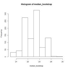
> median(mpg) # The actual sample median is 22.75;
bootstrap medians range
[1] 22.75 # from 20.5 to 25.0.
> sd(median_bootstrap)
[1] 0.7661376 # The bootstrap estimator of SD(median) is
0.7661376.
(4b) Bootstrap confidence interval
# The histogram above shows the distribution of
a sample median. We can find its (α/2)-quantile and
(1-α/2)-quantile. They estimate the true
quantiles that embrace the sample median with probability (1-α).
> alpha=0.05;
quantile( median_bootstrap, alpha/2 )
2.5%
21
> quantile(
median_bootstrap, 1-alpha/2 )
97.5%
24
# A bootstrap confidence interval for the
population median is [21, 24].
(4c) R package “boot”
# There is a special bootstrap tool in R package
“boot”.
# To use it for the same problem, we define a
function that computes a sample median for a given subsample…
> median.fn =
function(X,subsample){
+ return(median(X[subsample]))
+ }
# For example, here is a sample median for a
small subsample of size 10 without replacement…
> median.fn( mpg, sample(n,10)
)
[1] 24.95
# If the subsample is the whole sample, with all
its indices, we get our original sample median…
> median.fn( mpg, )
[1] 22.75
# Then we apply this function to many bootstrap
samples (R is their number) and summarize the obtained statistics…
> library (boot)
> boot( mpg, median.fn, R=10000 )
ORDINARY NONPARAMETRIC BOOTSTRAP
Call:
boot(data = mpg, statistic = median.fn, R = 10000)
Bootstrap Statistics :
original bias
std. error
t1* 22.75 -0.1406 0.7687722
# The bootstrap estimate of the standard
deviation of a sample median is 0.7687722, and the bootstrap estimate of the bias is -0.1406. If we run the same
command again, we might get somewhat different estimates, because the bootstrap
method is based on random resampling.
> boot( mpg,
median.fn, R=10000 )
original bias
std. error
t1* 22.75 -0.13368 0.7727318
> boot( mpg,
median.fn, R=10000 )
original bias
std. error
t1* 22.75 -0.13437 0.7617304
(4d) Another problem – find a bootstrap estimate
of the standard deviation of each regression coefficient
# Define a function returning regression intercept
and slope…
> slopes.fn =
function( dataset, subsample ){
+ reg = lm( mpg ~
horsepower, data=Auto[subsample, ] )
+ beta = coef(reg)
+ return(beta)
+ }
> boot( Auto,
slopes.fn, R=10000 )
Bootstrap Statistics :
original bias
std. error
t1* 39.9358610 0.0329999048
0.857890744
t2* -0.1578447 -0.0003929433 0.007444107
# We got bootstrap estimates, Std(intercept) =
0.85789, Std(slope) = 0.007444.
# Actually, this can be obtained easily, and
without bootstrap…
> summary( lm( mpg ~ horsepower, data=Auto )
)
Coefficients:
Estimate Std.
Error t value Pr(>|t|)
(Intercept) 39.935861
0.717499 55.66 <2e-16 ***
horsepower -0.157845 0.006446
-24.49 <2e-16 ***
# But…. Why are the bootstrap estimates of
standard errors higher than the ones obtained by regression formulae? Random
variation due to bootstrapping? Let’s try bootstrap a few more times.
> boot( Auto,
slopes.fn, R=10000 )
original bias
std. error
t1* 39.9358610 0.0366632516
0.864274619
t2* -0.1578447 -0.0003676081 0.007459809
> boot( Auto,
slopes.fn, R=10000 )
original bias
std. error
t1* 39.9358610 0.024793987
0.866532993
t2* -0.1578447 -0.000309597 0.007501155
> boot( Auto, slopes.fn,
R=10000 )
Bootstrap Statistics :
original bias
std. error
t1* 39.9358610 0.0411404502
0.868404735
t2* -0.1578447 -0.0004208256 0.007500111
# A comment about discrepancy with the
standard estimates. Bootstrap estimates are pretty close to each other.
They should be, because each of them is based on 10,000 bootstrap samples.
However, the bootstrap standard errors of slopes are still a little higher than
the estimates obtained by the standard regression analysis. The book explains
this phenomenon by a number of assumptions that the standard regression
requires. In particular, nonrandom predictors X and a constant variance of
responses Var(Y) = σ2. Bootstrap is a nonparametric procedure,
it is not based on any particular model. Thus, it can account for the variance
of predictors. Here, “horsepower” is the predictor, and it is probably random.
Since some of the standard regression
assumptions are questionable here, the bootstrap method for estimating standard
errors is more reliable.